-
Notifications
You must be signed in to change notification settings - Fork 7
Transitional Wing
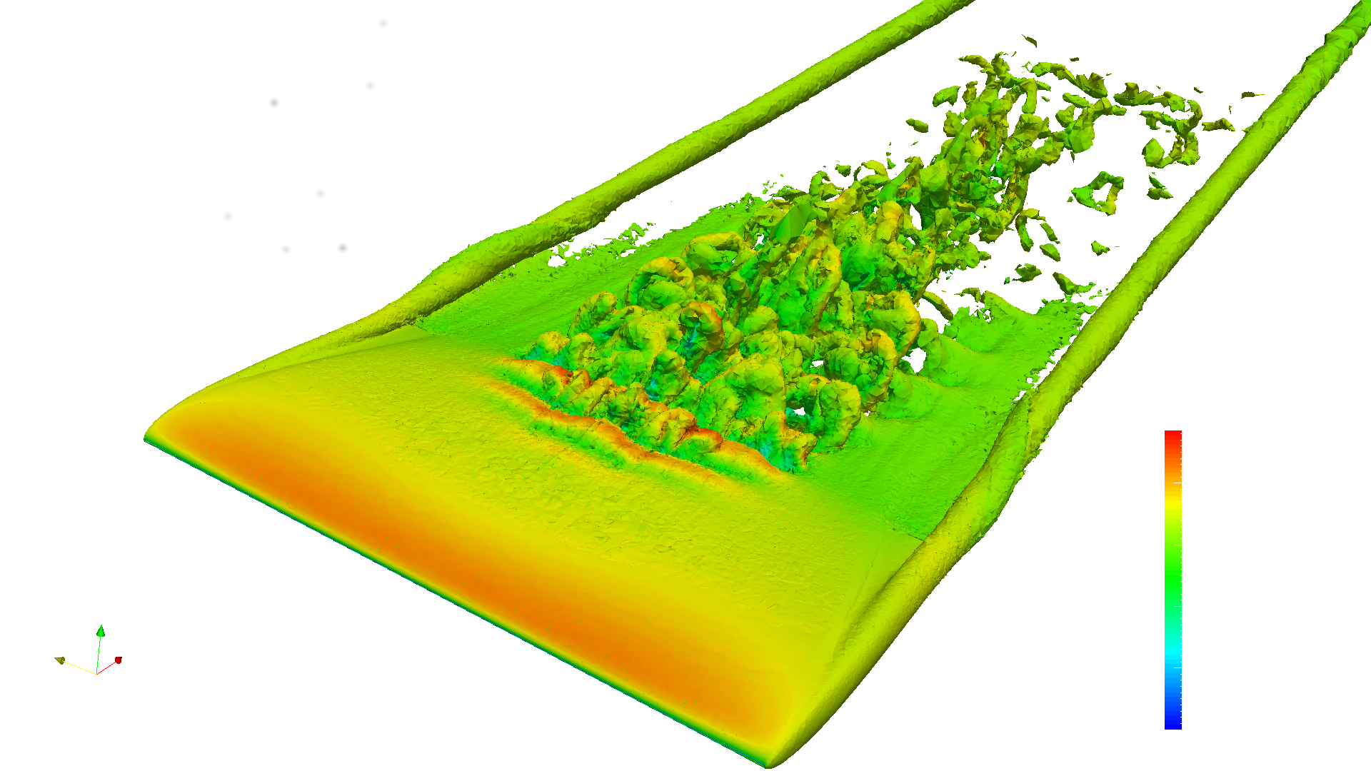
In this tutorial, we will compute the unsteady, transitional flow about a wing with AR=2 and a SD7003 airfoil section. The flow will be computed at a Mach number of 0.2 and a Reynolds number of 20,000. The root directory for this case is Tutorials/Unsteady_Wing_Navier-Stokes. Please be aware that this case will require approximately 60GB of memory and take approximately 12 hours to compute using 16 processors.
The geometry definition for this case is contained in the file SD7003Regtangular.stp. The GMSH configuration file SD7003Rectangular.geo is duplicated below.
fflc = 10.0;
surf_len = 0.04;
lete_factor = 0.25;

Mesh.CharacteristicLengthMax = fflc;
Mesh.CharacteristicLengthExtendFromBoundary = 0;
Mesh.SaveParametric = 1;
Merge "SD7003Rectangular.stp";


Mesh.Algorithm = 7;


Physical Line(0) = {1:29};

Physical Surface(6) = {1:6};
Physical Surface(7) = {7:14};

Delete{ Volume{1:2}; }

Reverse Surface{7:14};

Surface Loop(100) = {1:6};
Surface Loop(101) = {7:14};

Volume(1) = {100,-101};
Physical Volume(0) = {1};


Field[2] = Box;
Field[2].VOut = fflc;
Field[2].VIn = 0.5*surf_len;
Field[2].XMax = 1.02;
Field[2].XMin = 0.98;
Field[2].YMax = 2.02;
Field[2].YMin = 1.6;
Field[2].ZMax = 0.35;
Field[2].ZMin = -0.01;

Field[5] = Box;
Field[5].VOut = fflc;
Field[5].VIn = surf_len;
Field[5].XMax = 1.1;
Field[5].XMin = -0.1;
Field[5].YMax = 1.1;
Field[5].YMin = -1.1;
Field[5].ZMax = 0.15;
Field[5].ZMin = -0.07;

Field[6] = Box;
Field[6].VOut = fflc;
Field[6].VIn = 0.75*surf_len;
Field[6].XMax = 3;
Field[6].XMin = 0.5;
Field[6].YMax = 0.6;
Field[6].YMin = -0.6;
Field[6].ZMax = 0.3;
Field[6].ZMin = -0.2;

Field[7] = Box;
Field[7].VOut = fflc;
Field[7].VIn = 1.5*surf_len;
Field[7].XMax = 5;
Field[7].XMin = -0.5;
Field[7].YMax = 1.2;
Field[7].YMin = -1.2;
Field[7].ZMax = 0.5;
Field[7].ZMin = -0.3;


Field[8] = Box;
Field[8].VOut = fflc;
Field[8].VIn = 4*surf_len;
Field[8].XMax = 12;
Field[8].XMin = -1;
Field[8].YMax = 1.3;
Field[8].YMin = -1.3;
Field[8].ZMax = 1.0;
Field[8].ZMin = -0.75;

Field[9] = Box;
Field[9].VOut = fflc;
Field[9].VIn = 5*surf_len;
Field[9].XMax = 2.5;
Field[9].XMin = -1.5;
Field[9].YMax = 1.3;
Field[9].YMin = -1.3;
Field[9].ZMax = 1.5;
Field[9].ZMin = -1.5;

Field[12] = Box;
Field[12].VOut = fflc;
Field[12].VIn = 0.5*surf_len;
Field[12].XMax = 1.01;
Field[12].XMin = -0.01;
Field[12].YMax = 1.04;
Field[12].YMin = 1.0;
Field[12].ZMax = 0.06;
Field[12].ZMin = -0.05;

Field[13] = Box;
Field[13].VOut = fflc;
Field[13].VIn = 0.5*surf_len;
Field[13].XMax = 1.01;
Field[13].XMin = -0.01;
Field[13].YMax = -1.0;
Field[13].YMin = -1.04;
Field[13].ZMax = 0.06;
Field[13].ZMin = -0.05;


Field[14] = Box;
Field[14].VOut = fflc;
Field[14].VIn = 1;
Field[14].XMax = 15;
Field[14].XMin = -5;
Field[14].YMax = 2;
Field[14].YMin = -2;
Field[14].ZMax = 5;
Field[14].ZMin = -5;

Field[15] = Box;
Field[15].VOut = fflc;
Field[15].VIn = 0.004;
Field[15].XMax = 1.01;
Field[15].XMin = 0.8;
Field[15].YMax = -0.999;
Field[15].YMin = -1.03;
Field[15].ZMax = 0.05;
Field[15].ZMin = -0.05;

Field[16] = Box;
Field[16].VOut = fflc;
Field[16].VIn = 0.004;
Field[16].XMax = 1.01;
Field[16].XMin = 0.8;
Field[16].YMax = 1.03;
Field[16].YMin = 0.999;
Field[16].ZMax = 0.005;
Field[16].ZMin = -0.005;

Field[20] = AttractorAnisoCurve;
Field[20].EdgesList = {14,25};
Field[20].NNodesByEdge = 1000;
Field[20].dMin = 0.008;
Field[20].dMax = 20;
Field[20].lMinNormal = 0.005;
Field[20].lMinTangent = surf_len;
Field[20].lMaxNormal = fflc;
Field[20].lMaxTangent = fflc;


Field[10] = Min;
Field[10].FieldsList = {5,6,7,8,9,12,13,14,20};


Field[4] = BoundaryLayer;
Field[4].FacesList = {7:14};
Field[4].hfar = fflc;
Field[4].hwall_n = 0.035;
Field[4].hwall_t = surf_len;
Field[4].thickness = 0.04;
Field[4].ratio = 1.0;

Background Field = 10;

BoundaryLayer Field = 4;
The process for generating the high order mesh will differ slightly from the previous examples, as we will have GMSH create a single-layer boundary layer mesh which MeshOpt will subdivide and make high order. Also note since the geometry file contains two volumes, we must delete them and define a single volume. The process for generating the high order mesh for this case is further detailed in a MeshOpt tutorial here.
The linear GMSH mesh is created using the following commend:
gmsh -3 -optimize -smooth 5 SD7003Rectangular.geo
The MeshOpt.config file for this case is:
CaseParameters{
	GMSHFileName = SD7003Rectangular.msh;
	STEPFileName = SD7003Rectangular.surfaces.full.stp;
	OutputFileName = SD7003RectangularBL.msh;
}

BLParameters{
	HasBL = true;
	NLayers = 7;
	GrowthRatio = 1.4;
}

HighOrderParameters{
	Order = 2;
	TargetMinQuality = 0.9;
}
Since GMSH created a boundary layer, we set HasBL = true. We can now create the high order mesh SD7003RectangularBL.msh with MeshOpt.
The FlowEDG configuration file for this case is:
Project{
	Name = Transitional_SD7003;
	Equation = Navier-Stokes;
	MeshFile = SD7003AirfoilBL.msh;
	Discretization = EDG;
	OptimizedNodeSpacing = true;
}

EquationParameters{
	gamma = 1.4;
	Pr = 0.72;
	Re = 2.0e4;
	M_inf = 0.2;
	U_inf = {0.997564050259824,0,0.069756473744125}; # alpha = 4 degrees
}

NonlinearSolverParameters{
	MaxIt = 50;
	RelTol = 1.0e-4;
	Type = Quasi-Newton;
}

LinearSolverParameters{
	RelTol = 1.0e-4;
	Restart = 50;
	MaxIt = 50;
}

UnsteadyParameters{
	SolveUnsteady = true;
	dt = 0.01;
	Nt = 1000;
	Integration = DIRK33;
#	Restart = true;
#	RestartTimestep = 0;
}

PostProcessingParameters{
#	PostProcessOnly = true;
#	ValuesToSave = rho M s |Vort|;
#	StartTimestep = 1000;
#	NRefinements = 2;
}
As in the sphere case, we choose to discretize with EDG, since it is more efficient than HDG for p=2. The time step is chosen to be 0.01, and we will compute the solution for 1000 time steps using a third-order-accurate time integration scheme. Assuming that we want to run using 16 MPI processes:
mpirun -np 16 FlowEDG
This case will take a large amount of resource to compute, and this will only increase with increasing order. This case can be run with p=3 using EDG, but will require approximately four times as much memory and time to compute. p=4 will require 12 times as many resources.
We will take a look at time step 1000 by following the post-processing procedure detailed in previous tutorials. Please be aware that if we refine each element two times, as in the above configuration file, ParaView will require approximately 30GB of memory. Below we visualize the transitional flow using an isosurface of entropy colored by Mach number.
